Principal Component Analysis (PCA) in Machine Learning: A Beginner-Friendly Guide
Machine learning often works with datasets that contain many features. Sometimes that is useful, but very often it creates problems: the data becomes harder to visualize, training takes longer, and...
Machine learning often works with datasets that contain many features. Sometimes that is useful, but very often it creates problems: the data becomes harder to visualize, training takes longer, and some features may carry overlapping information. This is where Principal Component Analysis (PCA) becomes very helpful.
PCA is one of the most widely used techniques for dimensionality reduction. It helps us reduce the number of features in a dataset while preserving as much useful information as possible. If you are new to machine learning, think of PCA as a smart way of compressing data without losing the important patterns.
In this blog, we will understand PCA from the ground up: what it is, why it is needed, how it works, the steps involved, and a simple example to make the idea clear.
# What Is PCA?
Principal Component Analysis (PCA) is an unsupervised machine learning technique used to transform a dataset with many features into a smaller set of new features called principal components.
These principal components are:
- Linear combinations of the original features.
- Ordered by how much variance they capture from the data.
- Mutually orthogonal, meaning they are uncorrelated with each other.
In simple words, PCA finds the directions in which the data varies the most and uses those directions to represent the data in fewer dimensions.
# A Simple Intuition
Imagine you have a set of points spread on a sheet of paper. If the points mostly lie along a diagonal line, then instead of describing each point using both the horizontal and vertical directions, you can describe it mostly using that diagonal direction. PCA finds exactly such important directions.
So instead of saying:
- Feature 1 = height
- Feature 2 = weight
- Feature 3 = age
- Feature 4 = income
PCA may create new features like:
- Principal Component 1
- Principal Component 2
- Principal Component 3
These new features summarize the original ones in a more compact way.
# Why Do We Need PCA?
Real-world datasets can have dozens, hundreds, or even thousands of features. Working with all of them can be difficult.
PCA helps because it can:
- Reduce the number of dimensions in the data.
- Remove redundant information.
- Speed up model training.
- Help visualize high-dimensional data in 2D or 3D.
- Reduce noise in some cases.
- Improve performance when features are highly correlated.
# Problems Caused by High Dimensions
When the number of features becomes large, several issues arise:
- Models may become computationally expensive.
- Data visualization becomes difficult.
- Some features may contain duplicate or correlated information.
- The model may suffer from the curse of dimensionality.
The curse of dimensionality means that as dimensions increase, data points become sparse, distances become less meaningful, and learning becomes harder.
# Core Idea of PCA
The central idea behind PCA is:
Find new axes for the data such that: * The first new axis captures the maximum variance. * The second new axis captures the next highest variance. * Each new axis is perpendicular to the previous ones.
These new axes are called principal components.
# Variance Matters
PCA assumes that directions with higher variance contain more useful information about the structure of the data.
- High variance means the data is spread out more in that direction.
- Low variance means the data changes very little in that direction.
PCA keeps directions with high variance and can discard directions with low variance.
# Important Terms You Should Know
Before going deeper, let us define a few important terms.
# 1. Feature
A feature is an input variable in the dataset.
Example:
- Height
- Weight
- Age
- Salary
# 2. Dimension
Each feature represents one dimension. If a dataset has 5 features, it is a 5-dimensional dataset.
# 3. Variance
Variance measures how spread out the data is.
If a feature changes a lot across samples, it has high variance.
# 4. Covariance
Covariance tells us how two features vary together.
- Positive covariance: both increase together.
- Negative covariance: one increases while the other decreases.
- Near-zero covariance: little relationship.
# 5. Eigenvectors and Eigenvalues
These are mathematical concepts used in PCA.
- Eigenvectors represent directions.
- Eigenvalues represent the amount of variance captured in those directions.
In PCA:
- Eigenvectors become the principal components.
- Eigenvalues tell us how important each principal component is.
Do not worry if these sound difficult. We will make them intuitive in the step-by-step process.
# How PCA Works Conceptually
Suppose you have two features:
- Study hours
- Exam score
These two may be strongly related. Students who study more often score more. So the two features may provide overlapping information.
PCA rotates the coordinate system to find a better set of axes:
- One axis captures the main trend in the data.
- The other captures the smaller variation around that trend.
If most of the information lies along the first axis, we may keep only that axis and remove the second. This reduces dimensions while preserving most of the useful information.
# Step-by-Step Process of PCA
Now let us understand how PCA is performed.
# Step 1: Collect the Dataset
Suppose the dataset has n samples and d features.
For example, 100 students and 4 features per student.
# Step 2: Standardize the Data
This is one of the most important steps.
Why?
Because features may have different scales. For example:
- Age may range from 18 to 60
- Salary may range from 20,000 to 100,000
If we apply PCA directly, large-scale features will dominate the result.
So we standardize each feature using:
z=σx−μ
Where:
- x is the original value
- μ is the mean
- σ is the standard deviation
After standardization:
- Mean becomes 0
- Standard deviation becomes 1
# Step 3: Compute the Covariance Matrix
The covariance matrix captures how features relate to one another.
If there are d features, the covariance matrix will be of size d×d.
For a dataset matrix X, the covariance matrix is:
Cov(X)=n−11XTX
This matrix shows:
- Diagonal values: variance of each feature
- Off-diagonal values: covariance between pairs of features
# Step 4: Compute Eigenvalues and Eigenvectors
Now we calculate the eigenvalues and eigenvectors of the covariance matrix.
- Eigenvectors give the directions of the principal components.
- Eigenvalues tell how much variance each component captures.
If a component has a larger eigenvalue, it captures more important information.
# Step 5: Sort the Principal Components
Sort the eigenvectors by descending eigenvalues.
This gives:
- First principal component: maximum variance
- Second principal component: next maximum variance
- Third principal component: next, and so on
# Step 6: Select the Number of Components
We do not always keep all components. We select only the top k components that explain most of the variance.
A common way is to use explained variance ratio:
Explained Variance Ratio=Sum of all eigenvaluesEigenvalue of component
If the first 2 components explain 95% of the variance, then we may keep only those 2 components.
# Step 7: Transform the Original Data
Finally, project the original standardized data onto the selected principal components.
This gives a new dataset with fewer dimensions.
If X is the standardized data and W contains the selected eigenvectors, then:
XPCA=XW
Now the data is represented using fewer features.
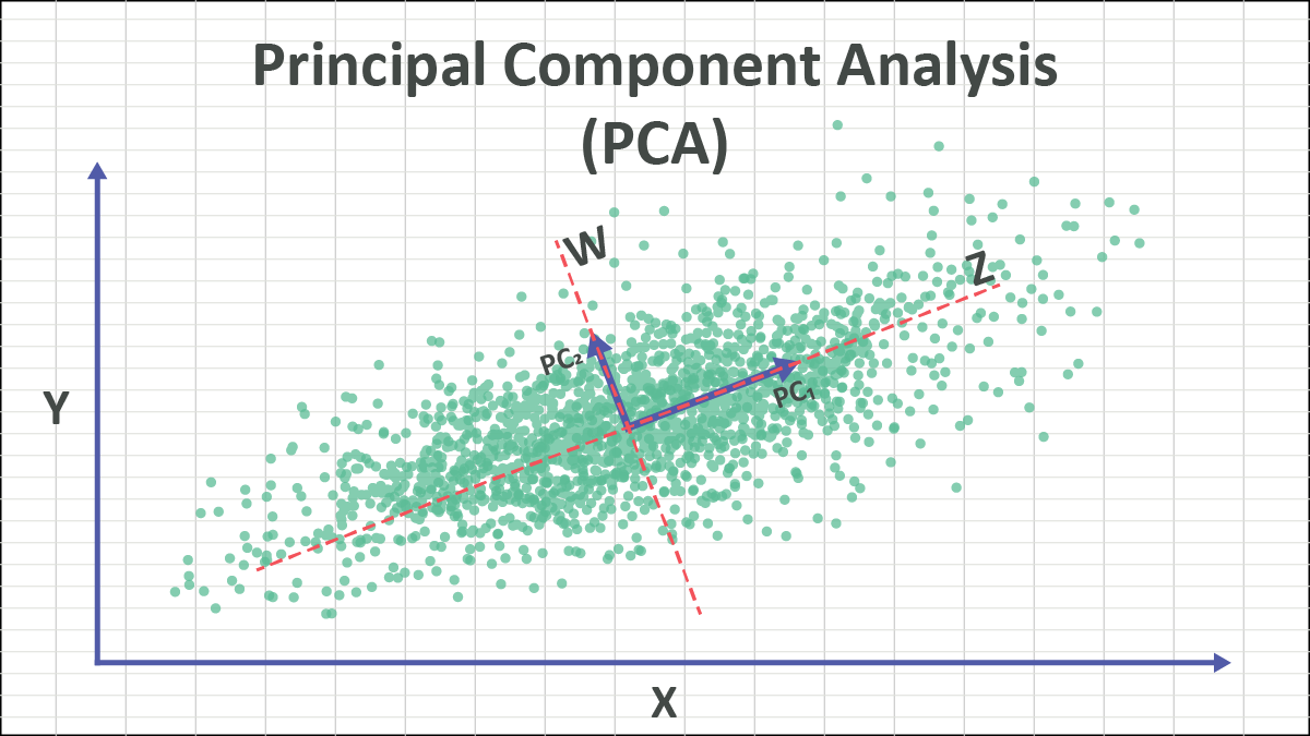
# Geometric Interpretation of PCA
PCA can be understood as a rotation of axes.
Originally, data is described along the original feature axes.
PCA changes the axes so that:
- The first axis goes in the direction of maximum spread.
- The second axis is perpendicular to the first and captures the next spread.
This is not just dropping columns. PCA creates new features that are combinations of old ones.
That is why PCA is called feature extraction, not merely feature selection.
# A Simple Numerical Example
Let us take a very simple dataset with two features:
- Hours studied
- Exam marks
| Student | Hours Studied | Exam Marks |
|---|---|---|
| A | 2 | 50 |
| B | 4 | 60 |
| C | 6 | 65 |
| D | 8 | 80 |
| E | 10 | 90 |
Here, exam marks increase as study hours increase. So both features are strongly correlated.
# What PCA Notices
PCA sees that:
- Most of the variation lies along one direction.
- The second direction contains much less information.
So instead of keeping both features, PCA may reduce them to one principal component that captures the overall academic performance trend.
# Intuitive Meaning
The first principal component may represent something like:
"General study-performance pattern"
The second principal component may represent:
"Small deviations from the usual pattern"
Since the second one carries less variance, we may ignore it.
# Real-Life Analogy
Imagine taking a photo of a tall building.
- A full 3D scene contains a lot of detail.
- But a 2D photo still captures the main structure.
Similarly, PCA reduces dimensions while trying to keep the most important structure of the data.
Of course, some information is lost, but the goal is to lose as little as possible.
# Explained Variance
One of the most important outputs of PCA is the explained variance ratio.
Suppose PCA gives the following:
- Principal Component 1 explains 75%
- Principal Component 2 explains 20%
- Principal Component 3 explains 5%
Then:
- Keeping only Component 1 preserves 75% of the information.
- Keeping first 2 components preserves 95% of the information.
This helps decide how many components to keep.
# When Should You Use PCA?
PCA is useful when:
- The dataset has many features.
- Features are correlated.
- You want to reduce training time.
- You want to visualize data in 2D or 3D.
- You want to remove noise or redundancy.
# Common Applications
- Image compression
- Face recognition
- Data visualization
- Preprocessing before classification or clustering
- Bioinformatics
- Finance and stock analysis
- Signal processing
# When PCA May Not Be Ideal
PCA is powerful, but not always the best choice.
Do not use PCA blindly when:
- Features are already few and interpretable.
- You need the original features for explanation.
- The relationships are strongly nonlinear.
- Variance does not necessarily mean importance.
PCA is a linear technique. If data lies on a nonlinear structure, methods like t-SNE, UMAP, or kernel PCA may work better.
# Advantages of PCA
- Reduces dimensionality.
- Removes multicollinearity.
- Improves computational efficiency.
- Helps visualization.
- Can reduce overfitting in some cases.
- Converts correlated variables into uncorrelated components.
# Limitations of PCA
- Components are harder to interpret than original features.
- PCA is sensitive to feature scaling.
- It may discard useful low-variance information.
- It assumes linear relationships.
- It is affected by outliers.
# PCA vs Feature Selection
Students often confuse these two ideas.
# Feature Selection
Feature selection chooses a subset of the original features.
Example:
- Keep height and weight
- Remove age and salary
# PCA
PCA creates entirely new features from combinations of original features.
Example:
- Principal Component 1 = 0.6×height+0.8×weight
- Principal Component 2 = another combination
So PCA does not simply pick columns. It transforms the data.
# PCA in Python Using Scikit-Learn
Here is a simple example in Python.
import numpy as np
import pandas as pd
from sklearn.preprocessing import StandardScaler
from sklearn.decomposition import PCA

# Sample dataset
data = {
    'Hours_Studied': [2, 4, 6, 8, 10],
    'Exam_Marks': [50, 60, 65, 80, 90]
}

df = pd.DataFrame(data)

# Step 1: Standardize the data
scaler = StandardScaler()
scaled_data = scaler.fit_transform(df)

# Step 2: Apply PCA
pca = PCA(n_components=1)
principal_components = pca.fit_transform(scaled_data)

# Convert result to DataFrame
pca_df = pd.DataFrame(data=principal_components, columns=['PC1'])

print("Transformed Data:")
print(pca_df)

print("\nExplained Variance Ratio:")
print(pca.explained_variance_ratio_)
# What This Code Does
- Loads a simple dataset.
- Standardizes the features.
- Applies PCA to reduce 2 features into 1 principal component.
- Prints the transformed data.
- Shows how much variance the retained component explains.
# Understanding the Output
The transformed values in PC1 are not directly "hours" or "marks". They are new values along the new principal axis.
If the explained variance ratio is very high, that means one component is enough to represent most of the information in the original two features.
# PCA on a Slightly Bigger Example
Suppose you have student data with these features:
- Study hours
- Attendance
- Assignment score
- Midterm score
- Final score
Many of these features may be correlated. A hardworking student tends to score well across multiple assessments.
PCA can compress these 5 features into perhaps 2 or 3 principal components such as:
- Overall academic performance
- Consistency vs exam strength
- Participation behavior
This reduced representation can then be used in:
- Clustering students
- Visualizing student groups
- Building faster predictive models
# How to Choose the Number of Components
There is no single rule, but common methods include:
# 1. Explained Variance Threshold
Keep enough components to preserve 90%, 95%, or 99% variance.
# 2. Scree Plot
A scree plot shows eigenvalues or explained variance for each component.
Look for the elbow point, where the gain starts decreasing sharply.
# 3. Based on Visualization Need
If you want to visualize high-dimensional data, reduce to 2 or 3 components.
# Mathematical Summary
Let the original standardized data matrix be X.
The PCA process is:
Standardize X
Compute covariance matrix:
C=n−11XTX
Find eigenvalues and eigenvectors of C
Sort eigenvectors by decreasing eigenvalues
Select top k eigenvectors to form matrix W
Transform data:
Z=XW
Where:
- X is original standardized data
- C is covariance matrix
- W contains selected principal directions
- Z is reduced-dimensional data
# Practical Tips for Beginners
If you are applying PCA in a real machine learning project, remember these points:
- Always scale the data before PCA.
- Do not apply PCA to the target variable.
- Start by checking explained variance ratio.
- Use PCA mainly when dimensionality is high or features are strongly correlated.
- Remember that transformed components are less interpretable.
# Interview-Style Questions on PCA
Here are a few common questions students may face:
# Is PCA supervised or unsupervised?
PCA is an unsupervised learning technique because it does not use target labels.
# Does PCA reduce overfitting?
It can help reduce overfitting by removing noisy or redundant features, but it is not guaranteed.
# Why do we standardize data before PCA?
Because PCA depends on variance, and features with larger scales can dominate if data is not standardized.
# Is PCA feature selection?
No. PCA is feature extraction because it creates new features.
# Can PCA be used for visualization?
Yes. PCA is often used to reduce data to 2 or 3 dimensions for plotting.
# Final Thoughts
PCA is one of the first dimensionality reduction techniques every machine learning student should learn. It is mathematically elegant, practically useful, and widely used in data preprocessing and visualization.
The main idea is simple:
- Find the directions where the data varies the most.
- Keep those directions.
- Drop the less important ones.
This allows us to represent complex high-dimensional data in a simpler and more compact way.
If you remember one thing, remember this:
PCA helps us keep the most important patterns in the data while reducing the number of features.
That makes machine learning workflows faster, cleaner, and often easier to understand.

About the Author
Dr. Himanshu Rai is an Assistant Professor in Computer Science & Engineering at SRM Institute of Science and Technology, specializing in Machine Learning, Artificial Intelligence, and Data Science. She is passionate about advancing research in computational intelligence and mentoring students.